Multi-Armed Bandits: Foundations

Multi-Armed Bandits and the Exploration–Exploitation Trade-off

If you have been around modern LLMs, you have probably heard of reinforcement learning. At its core, RL is an interaction loop: a learner chooses an action, receives feedback from the environment (reward), updates its rule for acting next time, and repeats. Much of today’s LLM finetuning to align with human preferences can be seen through this lens.

Unlike representation learning where the learner tries to "imitate" the data, RL forces the learner to interact with the environment. The central question in this interaction is how to balance exploration and exploitation. Should the learner take advantage of current knowledge and exploit the option that currently looks best to maximize immediate reward? Or should it take some risks to explore, potentially sacrificing short-term gains to improve knowledge and long-term performance? Too much greed misses better options; too much exploration wastes opportunities.

This fundamental tension between exploration and exploitation appears everywhere in sequential decision-making. Multi-armed bandits capture this trade-off in its simplest form: a single-state Markov decision process focused only on action selection under uncertainty. We now see applications of bandits across industries where information arrives in sequential manner. Examples range from ad placement, recommender systems, packet routing, to more theoretical settings like convex optimization and Brownian motion.

But what are bandit problems exactly?

A key early motivation came from clinical trials. William R. Thompson, in his 1933 paper, proposed assigning treatments adaptively using accumulating evidence, favoring promising options while still testing alternatives enough to learn.

The name “multi-armed bandit” came later. In the 1950s, Mosteller and Bush studied learning in animals and humans. Mice faced left/right choices in a T-shaped maze with uncertain rewards. For humans, they built a two-armed machine: each lever paid out randomly with unknown probabilities. The setup echoed the “one-armed bandit” slot machine, and the term “two-armed,” then “multi-armed,” bandit stuck.

A Classic Dilemma

Imagine you're playing a three-armed bandit machine. You've already pulled each lever several times and observed these payoffs (in dollars):

So far, Arm 1 averages $5, Arm 2 averages $0, and Arm 3 averages $7.50. You have 10 more pulls remaining. Do you stick with Arm 1 (reliable $5), gamble on Arm 3 (high variance but higher average), or give Arm 2 another chance? How do you balance exploiting what seems best versus exploring to learn more?

This illustrates the core dilemma in bandit problems: balancing exploration (trying uncertain options to gather information) and exploitation (using the currently best-performing option to maximize immediate reward).

Finite-Armed Stochastic Bandits: Warming Up

Bandit theory can quickly become intimidating as you could dive arbitrarily deep into measure theory, σ-algebras, or martingales. But that isn't necessary to grasp the core ideas. Instead, let's build intuition with the simplest meaningful setting: finite-armed stochastic bandits. This framework captures the essence of exploration versus exploitation while remaining concrete enough to analyze common solution strategies.

The problem statement is as follows: we have $K$ arms, where pulling arm $i$ at time $t$ yields reward $X_{i,t}$ drawn from an unknown distribution $\nu_i$ with mean $\mu_i$. The learner's goal is to minimize regret after $n$ rounds, which is the difference between the cumulative reward achieved by the learner, and that of an oracle that always pulls the optimal arm.

Why not evaluate a learner by raw cumulative reward $\sum_{t=1}^n X_t$?

• It is random: comparing policies requires a utility for the distribution of $S_n = \sum_{t=1}^n X_t$.
• The instance is unknown: a policy that maximizes $\mathbb{E}[S_n]$ for one set of rewards may perform poorly on another.

Regret avoids both by comparing the learner to an oracle that always pulls the best arm.

Define the optimal arm as $i^* = \arg\max_{i \in [K]} \mu_i$ with optimal mean $\mu^* = \mu_{i^*}$. The gap for arm $i$ is $\Delta_i = \mu^* - \mu_i$. After $n$ rounds, the cumulative regret is:

$$R_n = n\mu^* - \mathbb{E}\!\left[\sum_{t=1}^n X_{I_t, t}\right]$$

where $I_t$ is the arm selected at time $t$. Minimizing regret is equivalent to maximizing expected reward, but regret normalizes performance relative to the (unknown) optimum. If rewards were known, always pulling $i^*$ would give $R_n=0$.

This identity exposes the exploration–exploitation trade-off: each pull of a suboptimal arm incurs $\Delta_i$ expected loss. Good algorithms keep $\mathbb{E}[N_i(n)]$ small for large gaps while still exploring when gaps are small, targeting sublinear regret $R_n = o(n)$. The decomposition also provides a powerful framework for algorithm analysis. Instead of directly bounding the complex random quantity $R_n$, we can analyze each $\mathbb{E}[N_i(n)]$ separately.

Now let's formalize the problem setup.

First Steps: Explore-then-Commit

Before diving into principled algorithms, consider these simple heuristics:

• Greedy: Always play the arm with the highest empirical mean. This can get stuck on a suboptimal arm due to lack of exploration, leading to linear regret.
• Uniform exploration: Play all arms an equal number of times. This is pure exploration with no exploitation, also yielding linear regret.
• ε-greedy: With probability $1-\epsilon$, exploit by playing the empirically best arm; with probability $\epsilon$, explore by playing a random arm. This achieves $O(\log n)$ regret with proper tuning.

While ε-greedy can work reasonably well, it explores uniformly without considering confidence in the estimates. This motivates more sophisticated approaches.

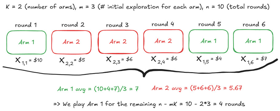
The first principled method we explore is called Explore-then-Commit. The approach is, explore each action/arm a fixed number of times ($m$), then exploit the knowledge by choosing the arm with the largest empirical payoff.

To analyze the regret of ETC, recall that $R_n = \sum_{i=1}^K \Delta_i \mathbb{E}[N_i(n)]$ from the regret decomposition above. Let's denote $i^* = \arg\max_i \mu_i$ as the optimal arm.

Intuitively, this bound captures the exploration–exploitation balance. Choosing a large $m$ means more time sampling every arm, so the first term (proportional to $m$) grows. Picking $m$ too small raises the chance of committing to a suboptimal arm, inflating the second term, which decreases only when $m$ is large enough to make the misidentification probability tiny.

To obtain a clean one-dimensional objective in $m$, specialize to the worst-case two-armed instance: set $K=2$ with $\Delta_1=0$ and denote $\Delta=\Delta_2$. Then only one suboptimal arm contributes and $$R_n \;\le\; m\,\Delta + (n-2m)\,\Delta\,\exp\!\left(-\tfrac{m\Delta^2}{4}\right) \;\le\; m\,\Delta + n\,\Delta\,\exp\!\left(-\tfrac{m\Delta^2}{4}\right),$$ since $n-2m \le n$. This is the scalar function we minimize to pick $m$.

Proof: In the first $mK$ rounds, the policy is deterministic, choosing each action exactly $m$ times. Subsequently it chooses a single action maximizing the average reward during exploration. Thus,

$$\mathbb{E}[N_i(n)] = m + (n - mK)\mathbb{P}(I_{mK+1} = i)$$

$$\leq m + (n - mK)\mathbb{P}\left(\hat{\mu}_i(mK) \geq \max_{j \neq i} \hat{\mu}_j(mK)\right)$$

The probability on the right-hand side is bounded by:

$$\mathbb{P}\left(\hat{\mu}_i(mK) \geq \max_{j \neq i} \hat{\mu}_j(mK)\right) \leq \mathbb{P}(\hat{\mu}_i(mK) \geq \hat{\mu}_{i^*}(mK))$$

This holds since beating all other arms implies beating the optimal arm $i^*$. Rewriting:

$$= \mathbb{P}(\hat{\mu}_i(mK) - \mu_i - (\hat{\mu}_{i^*}(mK) - \mu_{i^*}) \geq \Delta_i)$$

Then, we need to show that $\hat{\mu}_i(mK) - \mu_i - (\hat{\mu}_{i^*}(mK) - \mu_{i^*})$ is $\sqrt{2/m}$-subgaussian, which follows from standard subgaussian closure properties. Hence by Hoeffding's inequality:

$$\mathbb{P}(\hat{\mu}_i(mK) - \mu_i - \hat{\mu}_{i^*}(mK) + \mu_{i^*} \geq \Delta_i) \leq \exp\left(-\frac{m\Delta_i^2}{4}\right)$$

Substituting this into the expression for $\mathbb{E}[N_i(n)]$ and the regret decomposition gives the regret bound.

To choose the right $m$, we simplify to the basic two-arm instance: arm 1 is optimal ($\Delta_1=0$) and arm 2 is suboptimal with gap $\Delta_2=\Delta$. Then $K=2$ and the bound becomes $$R_n \;\le\; m\,\Delta + (n-2m)\,\Delta\,\exp\!\left(-\tfrac{m\Delta^2}{4}\right) \;\le\; m\,\Delta + n\,\Delta\,\exp\!\left(-\tfrac{m\Delta^2}{4}\right),$$ which is a one-dimensional function of $m$ that we can minimize explicitly.

The optimal choice is $m = \max\left\{1, \left\lceil \frac{4}{\Delta^2} \log\!\left(\frac{n\Delta^2}{4}\right) \right\rceil \right\}$ for gap $\Delta$. For the worst-case over gaps, this gives:

$$R_n \leq \Delta + C\sqrt{n}$$

where $C > 0$ is a universal constant. When $\Delta \leq 1$, we get $R_n \leq 1 + C\sqrt{n}$, or simply $R_n = O(\sqrt{n})$.

The previous choice of $m$ is close to the optimal choice, but it depends on both the unknown gap $\Delta$ and the horizon $n$. A standard alternative is to pick $m$ as a function of horizon $n$ only. For two 1-subgaussian arms, this yields a gap-free bound $R_n = O(n^{2/3})$.

Start from the two-arm bound derived above: $$R_n \;\le\; m\,\Delta + n\,\Delta\,\exp\!\left(-\tfrac{m\Delta^2}{4}\right).$$ For fixed $m$, upper bound the second term uniformly over $\Delta>0$. Let $g(\Delta)=\Delta\,\exp(-\tfrac{m\Delta^2}{4})$. Then $$g'(\Delta) = \exp(-m\Delta^2/4)\Big(1 - \tfrac{m\Delta^2}{2}\Big)=0\;\Rightarrow\; \Delta_* = \sqrt{\tfrac{2}{m}},$$ and $$\sup_{\Delta>0} g(\Delta) = g(\Delta_*) = \sqrt{\tfrac{2}{m}}\,\exp(-1/2) \;\le\; \frac{1}{\sqrt{m}}.$$ Hence, for all $\Delta>0$, $$R_n \;\le\; m\,\Delta + \sqrt{2}\,\exp(-1/2)\,\frac{n}{\sqrt{m}}.$$ Choosing $m = \lceil n^{2/3} \rceil$ gives $$R_n \;\le\; \Delta\,n^{2/3} + \sqrt{2}\,\exp(-1/2)\,n^{2/3} + O(\Delta),$$ which is at most $(\Delta + C)\,n^{2/3}$ for some constant $C$. In other words, $R_n = O(n^{2/3})$.

The Upper Confidence Bound (UCB) Algorithm

UCB elegantly addresses ETC's limitations by adaptively balancing exploration and exploitation. Instead of rigid phases, UCB constructs confidence intervals around arm means and selects the arm with highest upper confidence bound, a principle which we call optimism under uncertainty.

At time $t$, having selected arm $i$ a total of $N_i(t-1)$ times and observed empirical mean $\hat{\mu}_i(t-1)$, UCB selects:

$$I_t = \arg\max_{i \in [K]} \left( \hat{\mu}_i(t-1) + \sqrt{\frac{2\log t}{N_i(t-1)}} \right)$$

Exploitation vs. exploration: The term $\hat{\mu}_i(t-1)$ is the exploitation component, favoring arms that have produced large average rewards so far. The square-root term is the exploration bonus (confidence width): it is larger for arms with few samples ($N_i(t-1)$ small) and grows slowly with time through $\log(t)$, encouraging additional pulls until the estimate is accurate.

The expression inside the argmax is called the index of arm $i$. Index algorithms form a broad class of bandit strategies where each arm is assigned a numerical score (the index) based on its historical performance and uncertainty. The algorithm then simply selects the arm with the highest index at each round. Intuitively, this leads to sublinear regret because when the optimal arm's index overestimates its true mean, any suboptimal arm must achieve an index value exceeding the optimal arm's index to be selected. However, this can't happen too often as the learner continues to explore the environment and update its estimates.

The UCB algorithm is defined as follows:

UCB's regret analysis relies on optimism under uncertainty. The algorithm maintains confidence intervals such that with high probability, the true arm means lie within these intervals. When sufficient evidence accumulates (tight confidence intervals), the optimal arm will have the highest UCB and be selected most often.

The key lemma bounds how often UCB can select suboptimal arms:

Lemma: For any suboptimal arm $i$ with gap $\Delta_i > 0$, the number of times arm $i$ is selected satisfies:

$$\mathbb{E}[N_i(n)] \leq \frac{8\log n}{\Delta_i^2} + 1 + \frac{\pi^2}{3}$$

This leads to UCB's regret bound:

$$\mathbb{E}[R_n] \leq \sum_{i: \Delta_i > 0} \Delta_i \left( \frac{8\log n}{\Delta_i^2} + 1 + \frac{\pi^2}{3} \right) = \sum_{i: \Delta_i > 0} \left( \frac{8\log n}{\Delta_i} + O(1) \right)$$

Crucially, this scales as $O(\log n / \Delta_i)$ for each suboptimal arm, automatically adapting to problem difficulty. Arms with large gaps are quickly identified and avoided, while arms with small gaps are selected more often - exactly the desired behavior when arms have similar performance.

Optimality Concepts and Information Theory

To understand whether UCB is optimal, we need information-theoretic lower bounds. The fundamental question: what is the minimum regret any algorithm must accept when balancing exploration with exploitation?

The key insight comes from statistical hypothesis testing. Consider two bandit instances that are statistically "close" but have different optimal arms. An algorithm must distinguish between these instances, requiring sufficient data from each arm. This fundamental statistical requirement leads to unavoidable limits on learning efficiency.

Let $\mathcal{E} = \{\nu_1, \ldots, \nu_K\}$ be a bandit instance. The Lai–Robbins instance-dependent lower bound states that for any consistent algorithm and each suboptimal arm $i$:

$$\liminf_{n \to \infty} \frac{\mathbb{E}[N_i(n)]}{\log n} \geq \frac{1}{\text{KL}(\nu_i, \nu_{i^*})}.$$

For Gaussian rewards with unit variance, $\text{KL}(\mathcal{N}(\mu_i,1),\mathcal{N}(\mu^*,1)) = \Delta_i^2/2$, so asymptotically $\mathbb{E}[N_i(n)] \gtrsim \frac{2\log n}{\Delta_i^2}$. This quantifies instance difficulty via KL; problems with many small gaps are inherently harder.

The information-theoretic approach uses the Kullback-Leibler (KL) divergence between reward distributions. For distributions $P$ and $Q$:

$$\text{KL}(P, Q) = \int p(x) \log \frac{p(x)}{q(x)} dx$$

KL divergence measures the difficulty of distinguishing between distributions. Smaller KL divergence means harder discrimination, requiring more samples.

The change-of-measure technique relates regret to KL divergence. Consider an algorithm $\pi$ and two bandit instances $\mathcal{E}$ and $\mathcal{E}'$ differing only in arms $i$ and $j$. If instance $\mathcal{E}$ has optimal arm $i$ and instance $\mathcal{E}'$ has optimal arm $j$, then:

$$\mathbb{E}_{\mathcal{E}}[N_j(n)] \cdot \text{KL}(\nu_j, \nu_j') + \mathbb{E}_{\mathcal{E}}[N_i(n)] \cdot \text{KL}(\nu_i, \nu_i') \geq \text{kl}(\epsilon, 1-\epsilon)$$

where $\epsilon$ is the probability of misidentifying the optimal arm, and $\text{kl}(p,q) = p\log(p/q) + (1-p)\log((1-p)/(1-q))$ is the binary KL divergence.

This inequality captures the fundamental statistical trade-off: to achieve low error probability $\epsilon$ in arm identification, we must pull arm $i$ many times (if $\text{KL}(\nu_i, \nu_i')$ is small) or pull arm $j$ many times (if $\text{KL}(\nu_j, \nu_j')$ is small). This mathematical constraint reflects the statistical requirements for reliable learning.

More Information Theory and Minimax Lower Bounds

The minimax lower bound provides the worst-case regret any algorithm must suffer. It's derived by constructing a particularly challenging family of bandit instances.

Theorem (Minimax Lower Bound): For any algorithm and horizon $n \geq K$:

$$\inf_{\pi} \sup_{\mathcal{E}} \mathbb{E}_{\mathcal{E}}^{\pi}[R_n] \geq c\,\sqrt{K n}$$

for a universal constant $c>0$. One standard construction takes $K-1$ arms with mean $1/2 - \Delta$ and one arm with mean $1/2 + \Delta$, with $\Delta$ on the order of $\sqrt{K/n}$.

The proof uses Fano's inequality, a fundamental result in information theory. For a parameter estimation problem with $M$ hypotheses:

$$\mathbb{P}[\hat{\theta} \neq \theta] \geq 1 - \frac{I(X; \theta) + \log 2}{\log M}$$

where $I(X; \theta)$ is the mutual information between observations $X$ and parameter $\theta$.

Applied to bandits, Fano's inequality lower bounds the probability of misidentifying the optimal arm, which directly translates to regret. The construction ensures that:

1. The arms are sufficiently similar that many pulls are needed to distinguish them
2. The gaps are large enough that mistakes incur significant regret
3. The time horizon is short enough that perfect identification is impossible

Comparing with UCB's minimax regret bound of $O(\sqrt{K n \log n})$, we see that UCB is near-minimax optimal, suffering only an extra $\sqrt{\log n}$ factor. Algorithms like MOSS achieve minimax-optimal $O(\sqrt{K n})$ rates (up to constants), and KL-UCB attains optimal instance-dependent constants.

Instance Dependent Lower Bounds

While minimax bounds characterize worst-case performance, instance-dependent bounds reveal that UCB is actually optimal for specific problem instances.

Theorem (Lai-Robbins Lower Bound): For any consistent algorithm (one whose regret grows sublinearly), and any bandit instance with gaps $\Delta_i > 0$:

$$\liminf_{n \to \infty} \frac{\mathbb{E}[N_i(n)]}{\log n} \geq \frac{1}{\text{KL}(\nu_i, \nu_{i^*})}$$

Here, consistency means $\mathbb{E}[R_n] = o(n^{\alpha})$ for all $\alpha > 0$. The bound states that any reasonable algorithm must pull suboptimal arm $i$ at least $\frac{\log n}{\text{KL}(\nu_i, \nu_{i^*})}$ times.

This lower bound holds under standard regularity conditions (e.g., one-parameter exponential families with mild smoothness).

For Gaussian rewards with variance 1, $\text{KL}(\mathcal{N}(\mu_i, 1), \mathcal{N}(\mu^*, 1)) = \frac{(\mu^* - \mu_i)^2}{2} = \frac{\Delta_i^2}{2}$. This gives:

$$\liminf_{n \to \infty} \frac{\mathbb{E}[N_i(n)]}{\log n} \geq \frac{2}{\Delta_i^2}$$

Comparing with UCB's bound $\mathbb{E}[N_i(n)] \leq \frac{8\log n}{\Delta_i^2} + O(1)$, we see UCB achieves the optimal rate up to constants!

The Lai-Robbins proof employs the method of mixtures and change of measure. The key insight is that to distinguish between the true instance and a "confusing" alternative where arm $i$ is optimal, the algorithm must observe enough samples to resolve the statistical uncertainty.

Specifically, consider two instances:

• $\mathcal{E}$: True instance with optimal arm $i^*$
• $\mathcal{E}'$: Modified instance where arm $i$ is optimal (swapping means of arms $i$ and $i^*$)

If the algorithm pulls arm $i$ too few times, it cannot distinguish these instances, leading to suboptimal performance on one of them. The number of required samples is determined by the KL divergence between the arm distributions.

This establishes UCB as an optimal algorithm for the stochastic bandit problem, achieving both minimax optimality (up to log factors) and instance-dependent optimality.

Looking Ahead

We've established the foundational elements of bandit theory: the exploration-exploitation trade-off, algorithms like ETC and UCB for optimal arm selection, and the information-theoretic limits that govern learning. Key takeaways include:

• Regret decomposes as $\sum_i \Delta_i \mathbb{E}[N_i(n)]$, quantifying loss from selecting suboptimal arms
• UCB achieves optimal instance-dependent regret through adaptive confidence intervals, embodying optimism under uncertainty
• Information theory provides fundamental limits on how quickly we can identify optimal arms
• Instance-dependent regret can scale as $\sum_{i:\Delta_i>0} O(\log n/\Delta_i)$; worst-case minimax regret scales as $\Theta(\sqrt{K n})$.

This foundation prepares us for advanced topics. In Part 2, we'll explore adversarial settings where rewards can adapt to our actions, contextual bandits that incorporate side information, and structured approaches where rewards have known relationships. In Part 3, we'll dive into modern theory including sparse linear bandits, refined statistical bounds, and the elegant duality between Bayesian and frequentist approaches.

The mathematical machinery we've developed - concentration inequalities, confidence sets, information-theoretic arguments - forms the backbone of modern bandit algorithms, extending from simple comparisons to complex structured problems.

References

• Thompson, W. R. (1933). On the likelihood that one unknown probability exceeds another in view of the evidence of two samples. Biometrika, 25(3/4), 285-294.
• Lai, T. L., & Robbins, H. (1985). Asymptotically efficient adaptive allocation rules. Advances in Applied Mathematics, 6(1), 4-22.
• Auer, P., Cesa-Bianchi, N., & Fischer, P. (2002). Finite-time analysis of the multiarmed bandit problem. Machine Learning, 47(2-3), 235-256.
• Bubeck, S., & Cesa-Bianchi, N. (2012). Regret analysis of stochastic and nonstochastic multi-armed bandit problems. Foundations and Trends in Machine Learning, 5(1), 1-122.
• Lattimore, T., & Szepesvári, C. (2020). Bandit Algorithms. Cambridge University Press.
• Garivier, A., & Cappé, O. (2011). The KL-UCB algorithm for bounded stochastic bandits and beyond. COLT, 359-376.
• Berry, D. A., & Fristedt, B. (1985). Bandit Problems: Sequential Allocation of Experiments. Chapman and Hall.
• Thall, P. F., & Wathen, J. K. (2007). Practical Bayesian adaptive randomisation in clinical trials. European Journal of Cancer, 43(6), 859-866.